iOS versus Android: plotting tweet location heat maps with Twython
- 24 minsIn this post: creating a Twitter ‘app’; drinking from the Twitter firehose; an exotic projection; binning; blurring; a dubious preference metric.
Twitter recently retired their “version 1” API. It seems a good point, therefore, to learn both how to interact with their new “version 1.1” API and to see what sort of data Twitter lets you get on individual tweets. As usual for most of my little ‘learn how to do $$x$$’ projects, I’m going to reach for IPython. The code in this post is available in an IPython notebook (GitHub gist).
After a little Googling, I determined that twython looked to be a good choice for playing with Twitter. Not only is it, apparently, still maintained but it also has a plethora of Stack Overflow answers about it should I get stuck.
The Twitter API and OAuth2
The Twitter Application Programming Interface (API) is a service provided by Twitter which, perhaps unsurprisingly, provides an interface which allows you to program your own applications. (I believe the cool kids now refer to applications as ‘apps’.) Using the Twitter API, in essence, lets your program pretend to Twitter that they are a particular Twitter user. Usually this is to allow posting tweets, or reading a user’s timeline. Obviously there are some questions about security:
- How does Twitter know which app is trying to use the API? And how can it allow or disallow it?
- How does the user know which app is trying to use the API? And how can they allow or disallow it?
- How does the application know when both Twitter and the user have given permission?
- How does the application convince Twitter it’s got permission when the app uses the API?
Twitter decided to answer these questions by mandating that it’s API use something called OAuth2. This is a little dance that your app must perform to convince Twitter of who it is and that the user wants it. The process is fairly simple:
- The app and Twitter share a secret. This secret is used to convince Twitter that it’s talking to an application it knows.
- Twitter sends the app a link to a page dangling off api.twitter.com which the user should be directed to.
- The user is asked by Twitter if they trust the app and, if necessary, to sign in with their username and password.
- Twitter generates a new secret and it is passed back to the app.
- The app uses this secret from now on to a) prove who it is and b) prove the user allowed it.
Notice that the user’s username and password are never typed into the app. This is intended to stop malicious apps emailing Twitter usernames and passwords to the Bad Guys. (This is a very slimmed down description of OAuth, by the way, I’d read up on it if you’re interested in exactly how it works.)
Doing the dance in Python
So, let’s dive staight in and see how that dance is performed using twython. Firstly, you’ll need to create a new application on Twitter’s developers’ site. You’ll need a Twitter account to do this. When you’ve created the application, you’ll be given a page of OAuth settings like this:
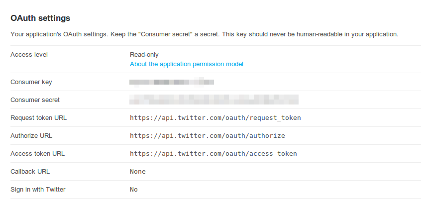
I’ve blanked out the consumer ker and consumer secret here. I created a credentials.py file with the credentials pasted in as follows:
CONSUMER_KEY = 'supersecretkey'
CONSUMER_SECRET = 'supersecretsecret'
(Obviously these are not my application’s actual credentials!) We can start using the Twitter API by importing twython and creating a Twitter object. After we do this, we ask Twitter for some authentication tokens we can use for the current connection:
from twython import Twython
from credentials import CONSUMER_KEY, CONSUMER_SECRET
twitter = Twython(CONSUMER_KEY, CONSUMER_SECRET)

# Start dancing...
auth = twitter.get_authentication_tokens()
OAUTH_TOKEN = auth['oauth_token']
OAUTH_TOKEN_SECRET = auth['oauth_token_secret']
twitter = Twython(CONSUMER_KEY, CONSUMER_SECRET, OAUTH_TOKEN, OAUTH_TOKEN_SECRET)
At this point we’re at stage 1 of the dance: Twitter knows who we are but not which user we want to act on behalf of. The user, also, doesn’t know what we’re up to. We now need to get our user to visit a particular URL, sign in and authenticate our app. Luckily Python has the smarts included to open the user’s web-browser at a particular URL:
import webbrowser
webbrowser.open_new_tab(auth['auth_url'])
If all has gone well, Twitter’s authorisation page should pop up.
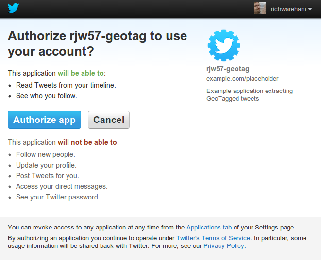
You want to use your own application, I presume, and so after clicking ‘Authorize [sic] app’ we get a PIN:
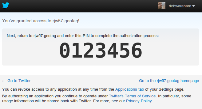
This PIN is the secret needed to get to the final stage of the dance: convincing Twitter that we are who we say we are, the user is aware of us and that they’ve allowed us to do the things we’re going to do.
PIN = '0123456'
final_step = twitter.get_authorized_tokens(PIN)
The final_step variable is a dictionary which holds the authentication tokens we should use from now on:
OAUTH_TOKEN = final_step['oauth_token']
OAUTH_TOKEN_SECRET = final_step['oauth_token_secret']
twitter = Twython(CONSUMER_KEY, CONSUMER_SECRET, OAUTH_TOKEN, OAUTH_TOKEN_SECRET)
Congratulations! We’re now fully authenticated with Twitter. Let’s prove this by dumping a JSON representation of the latest tweet by the Internet’s darling Stephen Fry:
import json
print(json.dumps(twitter.get_user_timeline(screen_name='stephenfry')[0], indent=2))
which, at the time of writing, resulted in this:
{
  "contributors": null,
  "truncated": false,
  "text": "@russellcrowe Perfect choice. Great cricketer & cricketing brain. Is going to make the series all the better. Brilliant Jor-El by the way",
  "in_reply_to_status_id": 349302248628682752,
  "id": 349304966269239299,
  "favorite_count": 39,
  "source": "<a href=\"http://twitterrific.com\" rel=\"nofollow\">Twitterrific for Mac</a>",
  "retweeted": false,
  "coordinates": null,
  "entities": {
    "symbols": [],
    "user_mentions": [
      {
        "id": 133093395,
        "indices": [
          0,
          13
        ],
        "id_str": "133093395",
        "screen_name": "russellcrowe",
        "name": "Russell Crowe"
      }
    ],
    "hashtags": [],
    "urls": []
  },
  "in_reply_to_screen_name": "russellcrowe",
  "id_str": "349304966269239299",
  "retweet_count": 23,
  "in_reply_to_user_id": 133093395,
  "favorited": false,
  "user": {
    "follow_request_sent": false,
    "profile_use_background_image": false,
    "default_profile_image": false,
    "id": 15439395,
    "verified": true,
    "profile_text_color": "333333",
    "profile_image_url_https": "https://si0.twimg.com/profile_images/344513261579148157/ba4807791ef9cce28dc0d4aa2ce9372c_normal.jpeg",
    "profile_sidebar_fill_color": "48CCF4",
    "entities": {
      "url": {
        "urls": [
          {
            "url": "http://t.co/4Kht71pdlB",
            "indices": [
              0,
              22
            ],
            "expanded_url": "http://www.stephenfry.com/",
            "display_url": "stephenfry.com"
          }
        ]
      },
      "description": {
        "urls": []
      }
    },
    "followers_count": 5902987,
    "profile_sidebar_border_color": "FFFFFF",
    "id_str": "15439395",
    "profile_background_color": "A5E6FA",
    "listed_count": 55634,
    "profile_background_image_url_https": "https://si0.twimg.com/profile_background_images/797461062/0ec127e26ce9be73cdafb2afca999cd6.jpeg",
    "utc_offset": 0,
    "statuses_count": 16302,
    "description": "British Actor, Writer, Lord of Dance, Prince of Swimwear & Blogger. NEVER reads Direct Messages: Instagram - stephenfryactually",
    "friends_count": 51546,
    "location": "London",
    "profile_link_color": "1C83A6",
    "profile_image_url": "http://a0.twimg.com/profile_images/344513261579148157/ba4807791ef9cce28dc0d4aa2ce9372c_normal.jpeg",
    "following": null,
    "geo_enabled": true,
    "profile_banner_url": "https://pbs.twimg.com/profile_banners/15439395/1360662717",
    "profile_background_image_url": "http://a0.twimg.com/profile_background_images/797461062/0ec127e26ce9be73cdafb2afca999cd6.jpeg",
    "screen_name": "stephenfry",
    "lang": "en",
    "profile_background_tile": false,
    "favourites_count": 78,
    "name": "Stephen Fry",
    "notifications": null,
    "url": "http://t.co/4Kht71pdlB",
    "created_at": "Tue Jul 15 11:45:30 +0000 2008",
    "contributors_enabled": false,
    "time_zone": "London",
    "protected": false,
    "default_profile": false,
    "is_translator": false
  },
  "geo": null,
  "in_reply_to_user_id_str": "133093395",
  "lang": "en",
  "created_at": "Mon Jun 24 23:16:08 +0000 2013",
  "in_reply_to_status_id_str": "349302248628682752",
  "place": null
}
As you can see, there are far more than 140 characters in a tweet nowadays(!)
Drinking from the hose
Nestled in that JSON response was a geo field. If a tweet has a location associated with it then this will be a dictionary with a coordinates field which, in turn, contains a tuple givint the latitude and longitude of the tweet. (Although it’s not obvious, it is likely that this is measured relative to the WGS84 datum.) In addition the tweet has a source field which is set by the application posting the Tweet. We’ll use the heuristic that if this contains the word “Android” then the device posting is an Android device and if it contains “iOS”, “iPhone” or “iPad”, it’s an iOS device.
Twitter has a streaming API which let’s us be notified when a Tweet is made that matches some search criteria. This is exposed in twython via the TwythonStreamer class. Using the class is pretty straight-forward: override an on_success method to receive each tweet and an on_error method to handle errors. In this case we can make a simple little object which will record the co-ordinates of each tweet in two lists depending on the device:
from twython import TwythonStreamer

class SourceStreamer(TwythonStreamer):
    def __init__(self, *args):
        super(SourceStreamer, self).__init__(*args)
        self.coords = {
            'android': [], 'iOS': [],
        }

    def on_success(self, data):
        """If tweet has geo-information, add it to the list."""
        try:
            source = data['source']
            if 'Android' in source:
                self.coords['android'].append(data['geo']['coordinates'])
            elif 'iOS' in source or 'iPhone' in source or 'iPad' in source:
                self.coords['iOS'].append(data['geo']['coordinates'])
        except (AttributeError, KeyError, TypeError):
            pass

    def on_error(self, status_code, data):
        """On error, print the error code and disconnect ourselves."""
        print('Error: {0}'.format(status_code))
        self.disconnect()
Using this object is fairly simple with one little wrinkle: twython blocks a stream when running until the disconnect method is called on it. We therefore start the stream running in its own thread:
from threading import Thread

class StreamThread(Thread):
    def run(self):
        self.stream = SourceStreamer(
            CONSUMER_KEY, CONSUMER_SECRET, OAUTH_TOKEN, OAUTH_TOKEN_SECRET
        )
        self.stream.statuses.filter(locations='-180,-90,180,90')

t = StreamThread()
t.daemon = True
t.start()
If we ever want to stop this thread, we can so so by calling t.stream.disconnect().
Plotting a heat map
I’ve already covered some of the issues involved with loading map images in another article and so I won’t repeat myself here. Suffice it to say that I once again used foldbeam to generate a base map. I wanted a somewhat exotic projection since I’d be showing the whole world. The Gall-Peters projection is interesting in that it is nearly unique amongst map projections in having an “in popular culture” section on its Wikipedia page.
To cut a long story short, this is the magic incantation to foldbeam:
$ foldbeam-render \
    --proj '+proj=cea +lon_0=0 +lat_ts=45 +x_0=0 +y_0=0 +ellps=WGS84 +units=m +no_defs' \
    -l -14000000 -r 14000000 -b -8500000 -t 8700000 -w 1280 -o world-map-gall.tiff --aerial
The long string passed to the --proj option comes from a spatialreference.org entry. Specifically, it’s the Proj4 string linked to from that page. If you want, you can download the resulting map.
Before we go any further, we should make sure to import NumPy and matplotlib:
import numpy as np
from matplotlib.pyplt import *
Loading the map into Python is achieved via the usual GDAL incantation and I’ve also written a little convenience function which maps latitude and longitudes into pixel co-ordinates for the map:
from osgeo import gdal, osr
map_ds = gdal.Open('world-map-gall.tiff')
map_image = np.transpose(map_ds.ReadAsArray(), (1,2,0))
ox, xs, _, oy, _, ys = map_ds.GetGeoTransform()
map_extent = ( ox, ox + xs * map_ds.RasterXSize, oy + ys * map_ds.RasterYSize, oy )

map_proj = osr.SpatialReference()
map_proj.ImportFromProj4(
    '+proj=cea +lon_0=0 +lat_ts=45 +x_0=0 +y_0=0 +ellps=WGS84 +units=m +no_defs'
)

wgs84_proj = osr.SpatialReference()
wgs84_proj.ImportFromEPSG(4326)

wgs84_to_map_trans = osr.CoordinateTransformation(wgs84_proj, map_proj)

def coord_to_pixel(coords):
    """Transform a sequence of co-ordinates in latitude, longitude
    pairs into map pixel co-ordinates."""

    # Transfrom from lat, lngs -> lng, lats
    latlngs = np.array(coords)
    lnglats = latlngs[:,(1,0)]

    # Transform from lng, lats -> map projection
    map_coords = np.array(wgs84_to_map_trans.TransformPoints(lnglats))

    # Transform from map projection -> pixel coord
    map_coords[:,0] = (map_coords[:,0] - ox) / xs
    map_coords[:,1] = (map_coords[:,1] - oy) / ys

    return map_coords[:,:2]
A heat map is a record, per pixel, of how many ‘things’ are within that pixel. In our application, this will be the number of tweets. The process of dividing a possible range of values up into individual areas and then counting the number of times something is present in that area is exactly what one does when plotting a histogram. The ever-wonderful NumPy library has a function which nearly does exactly what we want: np.histogram2d:
def coord_histogram(coords, down_scale = 2):
    pixel_locs = coord_to_pixel(coords)
    histogram, _, _ = np.histogram2d(pixel_locs[:,1], pixel_locs[:,0],
        bins=[int(map_image.shape[0]/down_scale), int(map_image.shape[1]/down_scale)],
        range=[[0, map_image.shape[0]], [0, map_image.shape[1]]])
    return histogram
There are a couple of interesting things here. Firstly we add a down_scale parameter which divides the pixel co-ordinates on the map for each tweet by some number. This is because our heat map should be at a lower resolution than our map since we only have a few tweets available. The second thing is that we explicitly specify the number of bins and the range of values to match our map image. If we didn’t do this, the function would try to guess appropriate values which may not be correct. Let’s calculate a histogram for Android and iOS:
android = coord_histogram(t.stream.coords['android'])
ios = coord_histogram(t.stream.coords['iOS'])
We can plot the histogram directly via imshow. The spectral colour map is quite nice and, to my mind, reminiscent of weather maps showing rainfall intensity which seems appropriate:
imshow(np.sqrt(ios), cmap=cm.spectral)
We use np.sqrt to “squash” the range of values so that very large tweet counts do not swamp the smaller ones. Feel free to experiment with removing the square root and see what the effect is.
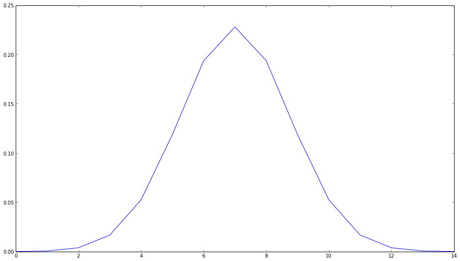
This isn’t bad but it’s a little bit “pointalist”. Let’s blur it with a Gaussian blur. We do this by convolving the image with a kernel. Luckily the scipy library comes with a handy one-dimensional Gaussian function:
from scipy.stats import norm
kern_row = norm.pdf(np.linspace(-4, 4, 15))
kern_row /= np.sum(kern_row)
plot(kern_row)
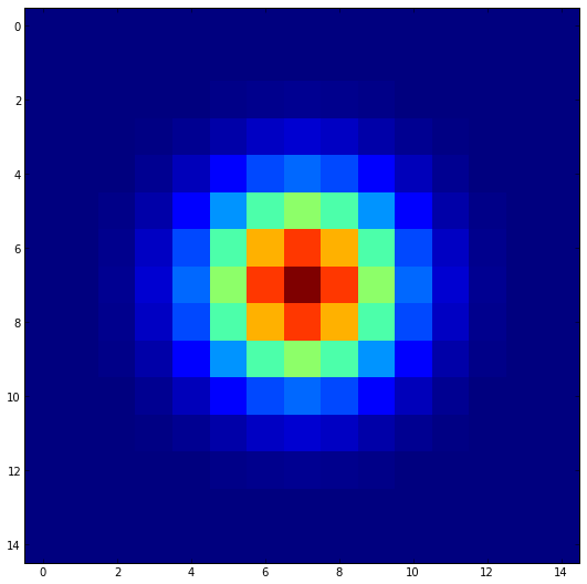
And, since a 2-d Gaussian is separable, making the 2-d version is just a case of taking the outer product:
kernel = np.outer(kern_row, kern_row)
imshow(kernel, interpolation='nearest')
Blurring the heat map is then pretty easy:
from scipy.signal import convolve2d
imshow(np.sqrt(convolve2d(android, kernel, mode='same')), cmap=cm.spectral)
axis('off')

Putting it all together, we can overlay the heat map atop the base map in two lines:
figure(figsize=(12,9))
imshow(map_image, extent=map_extent)
imshow(np.sqrt(convolve2d(android, kernel, mode='same')), extent=map_extent, alpha=0.5, cmap=cm.spectral)
axis('off')
title('Android usage as measured by Twitter ({0:,} tweets)'.format(int(android.sum())))
tight_layout()
savefig('android-usage.png')

figure(figsize=(12,9))
imshow(map_image, extent=map_extent)
imshow(np.sqrt(convolve2d(ios, kernel, mode='same')), extent=map_extent, alpha=0.5, cmap=cm.spectral)
axis('off')
title('iOS usage as measured by Twitter ({0:,} tweets)'.format(int(ios.sum())))
tight_layout()
savefig('ios-usage.png')
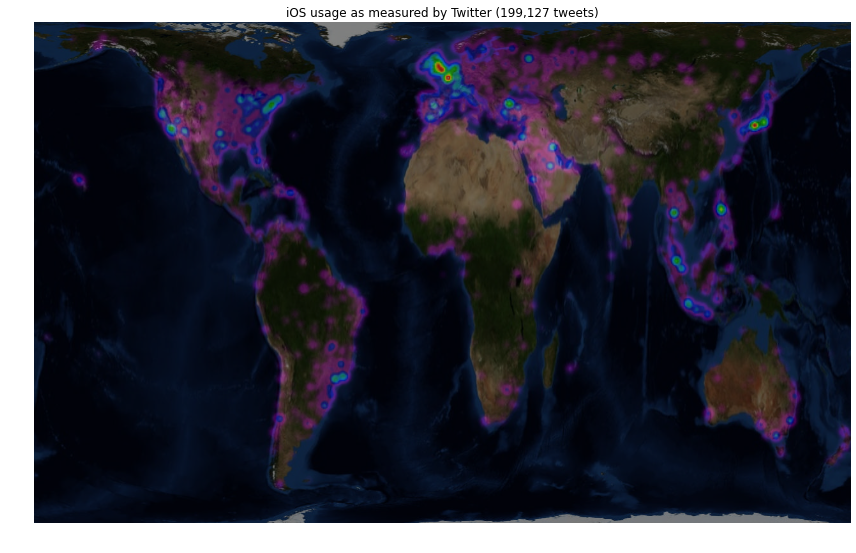

Now, bear in mind that these results were generated during the UK’s lunch time and so there’ll be a bias toward the UK and Western Europe. That being said quite a few things are obvious:
- The UK, Northern France and the low countries love iOS.
- Both Paris and London are clear hot spots.
- Moscow is clearly visible in the iOS map, but not Android.
- Spain loves Android.
- Everyone in Holywood has an iPhone.
- The usage of Android is more uniform with population in the US whereas iPhones are disproportionately used by people on the East and West coast population centres.
- Indonesia loves Android but is less embracing of iOS.
- Brazil looks to be equally favourable towards iOS and Android but Argentina loves the robot.
Finding preferences
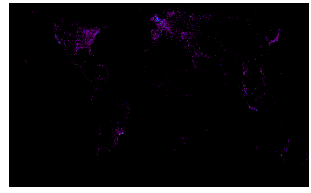
It would be interesting to plot some sort of ‘preference’ map showing which regions liked one device over another. Since we have a heat map for each device, the difference in heat maps should reveal areas of the world which favour one device over another. Matplotlib lets us call colourmap functions directly to get a coloured image out and below we make use of this to directly composite a heat map over the base map image. It also shows some tricks with colour bars:
figure(figsize=(12,6))

# Compute a preference matrix varying from -1 == iOS to +1 == Android
A = convolve2d(android/android.sum() - ios/ios.sum(), kernel, mode='same')
A /= max(A.max(), -A.min())

# Squash the *magnitude* of A by taking a square root
A = np.sign(A) * np.sqrt(np.abs(A))

# Show the base map
gca().set_axis_bgcolor('black')
imshow(map_image, extent=map_extent, alpha=0.5)

# Compute the coloured preference image and set alpha value based on preference
pref_cmap = cm.RdYlBu
pref_im = pref_cmap(0.5 * (A + 1))
pref_im[:,:,3] = np.minimum(1, np.abs(A) * 10)

# Draw preference image
imshow(pref_im, extent=map_extent, cmap=pref_cmap, clim=(-1,1))

# Draw a colour bar
cb = colorbar()
cb.set_ticks((-1, -0.5, 0, 0.5, 1))
cb.set_ticklabels(('Strong iOS', 'Weak iOS', 'No preference', 'Weak Android', 'Strong Android'))

# Set up plot axes, title and layout
gca().get_xaxis().set_visible(False)
gca().get_yaxis().set_visible(False)
title('Geographic preferences for Android vs. iOS')
tight_layout()

savefig('preferences.png')
The figure generated by this code is at the top of this post. Do we believe it? Well, the source is at least uninterested in whether iOS or Android is preferred in any one region but bear in mind that this result could well be biased by at least two effects:
- Different devices’ twitter clients may be more or less keen to report which device they’re on.
- iOS and Android users may differ in how much they want to geo-tag their tweets.
That being said, the results are quite pleasing.
Resources
- An IPython notebook and corresponding GitHub gist which has all the code in this post.
- The Twython documentation
- The Twitter developer documentation

Rich Wareham
You know, programming is fun!