Making a Little Planet Panorma using Python and Scikit Image
- 12 minsThis post is also available as an IPython notebook which may be downloaded or viewed online.
Recently I shared a post on G+ which had a Google “photosphere” transformed into the “little planet” projection. This post (and associated IPython notebook) will walk you through the way I created the planet image using scikit-image. This was my first steps with scikit-image since previously I had been using OpenCV. Unfortunately OpenCV is a bit of a pain to install and so I was looking for a pip-installable library with the functionality I required.
Loading the initial panorama
As usual, we need a little bit of boiler-plate to locad matplotlib and numpy. I’m also going to import the Pillow library for loading images (although I think scikit-image could do that).
# IPython magic to allow inline plots
%matplotlib inline

import os # for file and pathname handling functions
import matplotlib.pyplot as plt
import numpy as np
from PIL import Image

# Set the default matplotlib figure size to be a bit bigger than default
plt.rcParams['figure.figsize'] = (16,9)
On my phone, the photosphere is stored as a single JPEG file. Let’s use Pillow to load the image and display it via matplotlib:
pano = np.asarray(Image.open(os.path.expanduser('~/Downloads/PANO_20140927_124513.jpg')))
plt.imshow(pano)
<matplotlib.image.AxesImage at 0x7f91a1106090>
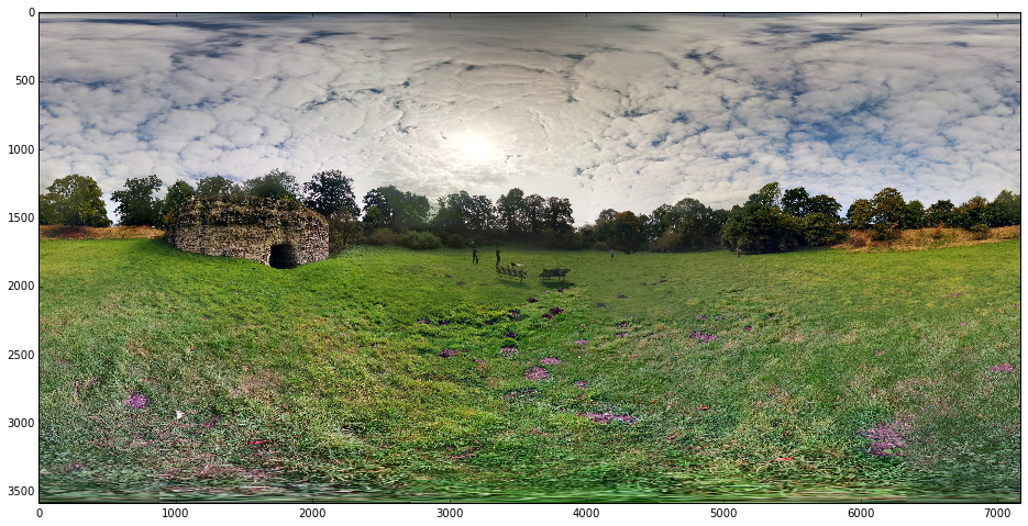
Beautiful. The next step is to work out how to warp this image.
Image warping via scikit-image
Looking at the appropriate section in the scikit-learn documentation, we see that there is a handy function called warp which will do exactly what we want. The function takes, amongst other inputs, the image to warp, the output image shape and a function which specifies the warp itself.
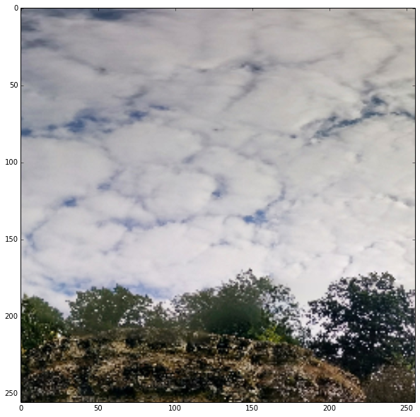
This function takes a N⨉2 array of (x,y) co-ordinates in the output image and turns them into a corresponding array of co-ordinates in the input image. Let’s just have a go at that using a very simple function which scales and shifts the co-ordinates:
from skimage.transform import warp

def scale_by_5_and_offset(coords):
    out = coords * 5
    out[:,0] += 1000
    out[:,1] += 300
    return out

plt.figure(figsize=(10,10)) # A square figure for square output
plt.imshow(warp(pano, scale_by_5_and_offset, output_shape=(256,256)))
<matplotlib.image.AxesImage at 0x7f917c93c610>
The “little planet” projection
The panorama we have is in the “equirectangular” projection which means that the y-co-ordinate represents the up-down angle and the x-co-ordinate represents the left-right angle. The little planet projection takes a different approach: the up-down angle is now specified by the distance from the centre of the image and the left-right angle is given by the angle from the horizontal in the image.
Given a particular output image shape, therefore, we can convert a co-ordinate in that image to a radius and angle, or 𝑟 and 𝜃 pair:
# What shape will the output be?
output_shape = (1080,1080) # rows x columns

def output_coord_to_r_theta(coords):
    """Convert co-ordinates in the output image to r, theta co-ordinates.
    The r co-ordinate is scaled to range from from 0 to 1. The theta
    co-ordinate is scaled to range from 0 to 1.

    A Nx2 array is returned with r being the first column and theta being
    the second.
    """
    # Calculate x- and y-co-ordinate offsets from the centre:
    x_offset = coords[:,0] - (output_shape[1]/2)
    y_offset = coords[:,1] - (output_shape[0]/2)

    # Calculate r and theta in pixels and radians:
    r = np.sqrt(x_offset ** 2 + y_offset ** 2)
    theta = np.arctan2(y_offset, x_offset)

    # The maximum value r can take is the diagonal corner:
    max_x_offset, max_y_offset = output_shape[1]/2, output_shape[0]/2
    max_r = np.sqrt(max_x_offset ** 2 + max_y_offset ** 2)

    # Scale r to lie between 0 and 1
    r = r / max_r

    # arctan2 returns an angle in radians between -pi and +pi. Re-scale
    # it to lie between 0 and 1
    theta = (theta + np.pi) / (2*np.pi)

    # Stack r and theta together into one array. Note that r and theta are initially
    # 1-d or "1xN" arrays and so we vertically stack them and then transpose
    # to get the desired output.
    return np.vstack((r, theta)).T
We’re now very nearly in a position to generate our first little planet picture. In our original panorama 𝑟=0 corresponds to the bottom of the picture (i.e. maximum y-co-ordinate) and 𝑟=1 corresponds to the top (i.e. a y-co-ordinate of zero). Similarly 𝜃=0 corresponds to an x-co-ordinate of 0 and 𝜃=1 corresponds to the maximum x-co-ordinate. We can write a function to convert these co- ordinates:
# This is the shape of our input image
input_shape = pano.shape

def r_theta_to_input_coords(r_theta):
    """Convert a Nx2 array of r, theta co-ordinates into the corresponding
    co-ordinates in the input image.

    Return a Nx2 array of input image co-ordinates.

    """
    # Extract r and theta from input
    r, theta = r_theta[:,0], r_theta[:,1]

    # Theta wraps at the side of the image. That is to say that theta=1.1
    # is equivalent to theta=0.1 => just extract the fractional part of
    # theta
    theta = theta - np.floor(theta)

    # Calculate the maximum x- and y-co-ordinates
    max_x, max_y = input_shape[1]-1, input_shape[0]-1

    # Calculate x co-ordinates from theta
    xs = theta * max_x

    # Calculate y co-ordinates from r noting that r=0 means maximum y
    # and r=1 means minimum y
    ys = (1-r) * max_y

    # Return the x- and y-co-ordinates stacked into a single Nx2 array
    return np.hstack((xs, ys))
Let’s test our mapping functions using the warp function:
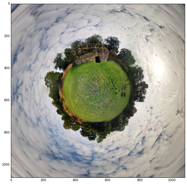
def little_planet_1(coords):
    """Chain our two mapping functions together."""
    r_theta = output_coord_to_r_theta(coords)
    input_coords = r_theta_to_input_coords(r_theta)
    return input_coords

plt.figure(figsize=(10,10))
plt.imshow(warp(pano, little_planet_1, output_shape=output_shape))
<matplotlib.image.AxesImage at 0x7f917c8ab2d0>
That’s not a bad first attempt but it would be nicer if we had a bit more horizon and a little less ground. That is to say we’d like to map 𝑟 a bit so that it increases quite rapidly to start with but flattens off a little. Usefully the square root function behaves a little like that:
rs = np.linspace(0, 1, 100)
plt.plot(rs, np.sqrt(rs))
[<matplotlib.lines.Line2D at 0x7f917c88e7d0>]
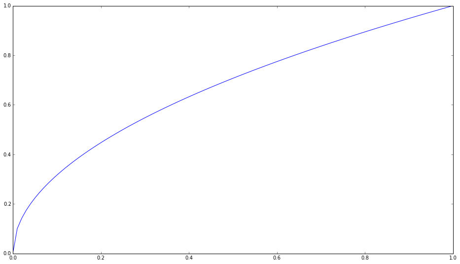
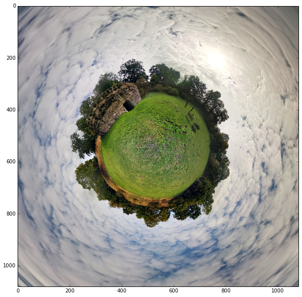
So let’s modify our little planet projection to take the square root of 𝑟:
def little_planet_2(coords):
    """Chain our two mapping functions together with modified r."""
    r_theta = output_coord_to_r_theta(coords)
    # Take square root of r
    r_theta[:,0] = np.sqrt(r_theta[:,0])
    input_coords = r_theta_to_input_coords(r_theta)
    return input_coords

plt.figure(figsize=(10,10))
plt.imshow(warp(pano, little_planet_2, output_shape=output_shape))
<matplotlib.image.AxesImage at 0x7f917c7eeb90>
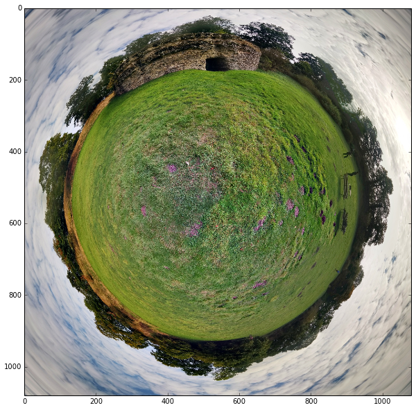
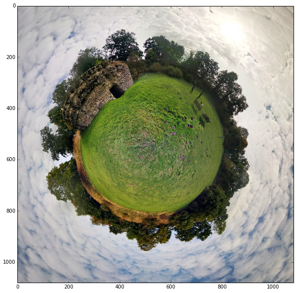
That’s better. The castle and trees look less warped. It would be nice to have the castle come out at a slightly different angle though. We can do that by shifting theta:
def little_planet_3(coords):
    """Chain our two mapping functions together with modified r
    and shifted theta.

    """
    r_theta = output_coord_to_r_theta(coords)

    # Take square root of r
    r_theta[:,0] = np.sqrt(r_theta[:,0])

    # Shift theta
    r_theta[:,1] += 0.1

    input_coords = r_theta_to_input_coords(r_theta)
    return input_coords

plt.figure(figsize=(10,10))
plt.imshow(warp(pano, little_planet_3, output_shape=output_shape))
<matplotlib.image.AxesImage at 0x7f917c7d4790>
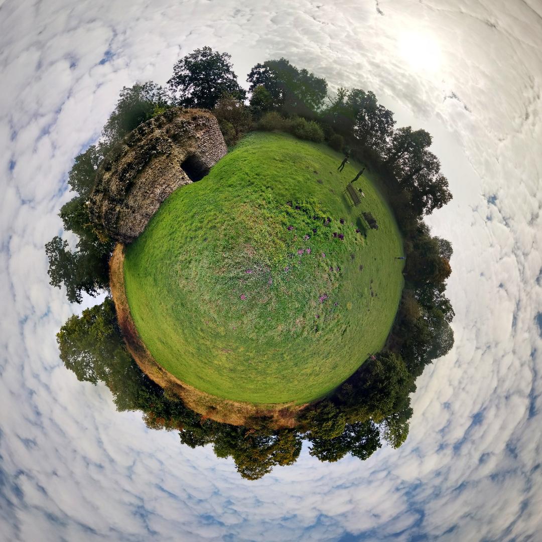
That’s nicer. There’s possibly a little too much sky so, finally, let’s just zooom in a bit by scaling $r$ down a bit:
def little_planet_4(coords):
    """Chain our two mapping functions together with modified and
    scaled r and shifted theta.

    """
    r_theta = output_coord_to_r_theta(coords)

    # Scale r down a little to zoom in
    r_theta[:,0] *= 0.75

    # Take square root of r
    r_theta[:,0] = np.sqrt(r_theta[:,0])

    # Shift theta
    r_theta[:,1] += 0.1

    input_coords = r_theta_to_input_coords(r_theta)
    return input_coords

plt.figure(figsize=(10,10))
plt.imshow(warp(pano, little_planet_4, output_shape=output_shape))
<matplotlib.image.AxesImage at 0x7f917c738290>
Saving the result
I’m happy with this image now. Let’s use Pillow to save the result:
# Compute final warped image
pano_warp = warp(pano, little_planet_4, output_shape=output_shape)

# The image is a NxMx3 array of floating point values from 0 to 1. Convert this to
# bytes from 0 to 255 for saving the image:
pano_warp = (255 * pano_warp).astype(np.uint8)

# Use Pillow to save the image
Image.fromarray(pano_warp).save(os.path.expanduser('~/Pictures/little-planet.jpg'))
IPython can display images directly fiven a filename. Let’s just check it saved correctly:
from IPython.display import Image as display_Image
display_Image(os.path.expanduser('~/Pictures/little-planet.jpg'))
Summary
In this post we gave a quick example of how to interactively play with an image and warp it from an equirectangular projection to the popular “little planet” projection.

Rich Wareham
You know, programming is fun!